On the limiting behaviour of the Uhlig 1997 Stochastic Volatility model

Uhlig (1997) proposed a VAR with stochastic volatility where precision, the inverse of variance, is given by a multiplicative process with beta innovations. The model lends itself to a high level of tractability since exact updating formulas are obtained. Lately I’ve been playing around with this model and found out some interesting aspects.

For the simple scalar case the model is as follows:

\[ y_t = \beta y_{t-1} + h_t^{-1/2}\epsilon_t, \ \ \epsilon_t \overset{iid}{\sim}\mathscr{N}(0,1) \\ h_{t+1} = h_t \mathscr{V}_t/\lambda, \ \ \mathscr{V}_t \overset{iid}{\sim}\mathscr{B}(\nu/2, 1/2) \] where \(h_1 \sim \mathscr{G}(s_0, \nu)\). The multiplicative process for precision can be analyzed in the light of results by Nelson (1990). The density of the beta innovation is given by:

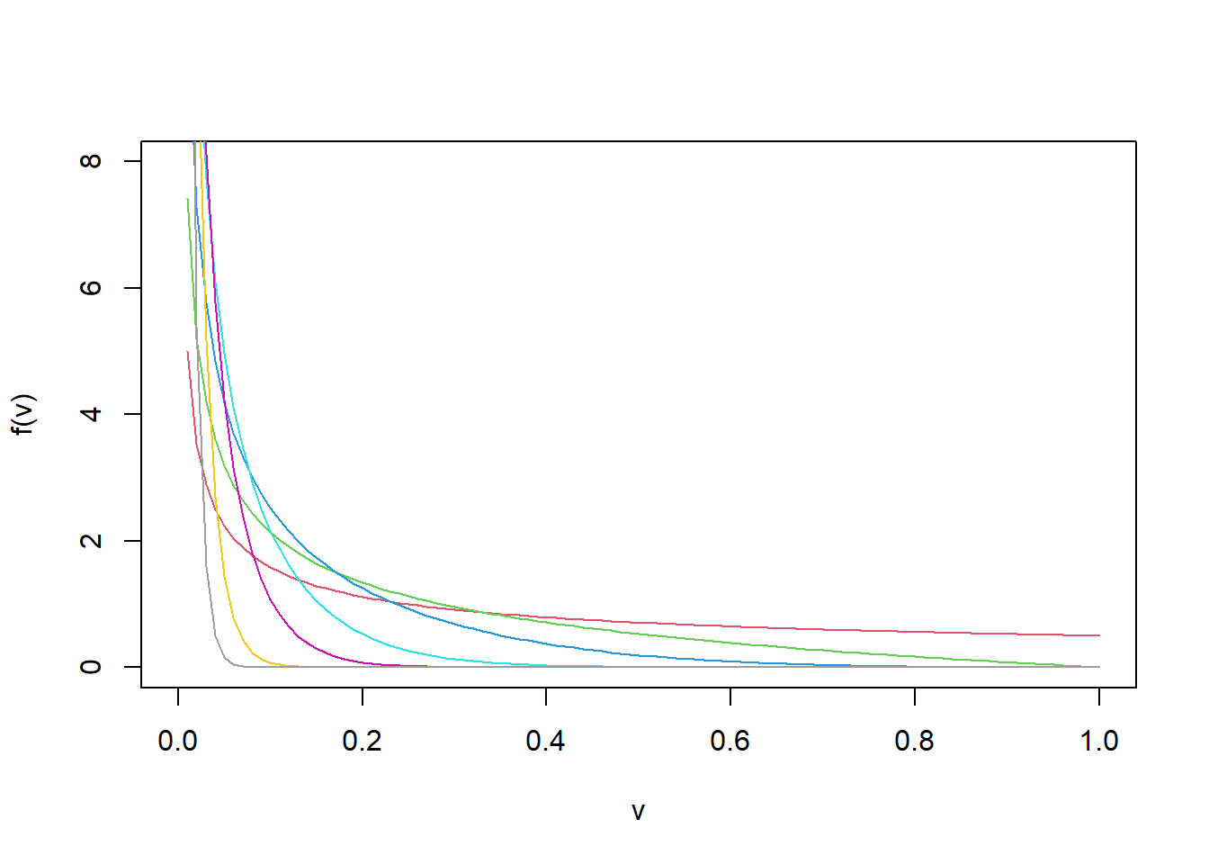
\[ f_\mathscr{V}(v) = \frac{\Gamma\left( \frac{\nu+1}{2} \right)}{\Gamma\left(\frac{1}{2}\right)\Gamma\left(\frac{\nu}{2}\right)}v^{\frac{1}{2}-1}(1-v)^{\frac{\nu}{2}-1} \]

Notice we can move \(h_t\) to the left, take logs and expectations, assuming the parameters to be known: \[ \mathbb{E}\left\{\ln\left(\frac{h_{t+1}}{h_t}\right) \right\} = \mathbb{E}\left\{ \ln\left( \mathscr{V}_t \right) \right\} - \ln(\lambda) \] This term is the average growth rate of \(h_t\), precision. If the term is positive, it will grow to \(+\infty\) almost surely. If the term is negative it will go to 0 almost surely. Therefore, it seems that the only ‘reasonable’ specification is to let this term be 0. In other words, pick \(\lambda\) such that \(\ln h_t\) is a random walk. This will be the case when \(\lambda = \exp\left( \psi\left( \frac{1}{2} \right) - \psi\left( \frac{\nu+1}{2} \right) \right)\); where \(\psi(\cdot)\) is the diagamma function. An interesting and relevant question about this process is the following: Does this model nest an homoskedastic model as a limiting case? Is there some set of parameters that would collapse the model to a standard Gaussian AR(1)?

In the words of Uhlig:

For \(\nu \rightarrow \infty\) one obtains a model where \(h_1\) is known a priori, \(h_1 = s_0^{-1}\), and \(h_{t+1} = h_t(\nu+1)/(\lambda(\nu+2))\). In other words, the model allows for the greater time variation in the prescision, the smaller the parameter \(\nu\).

Unfortunately I am not able to obtain this limiting case. The mode is not \((\nu+1)/(\nu+2) \rightarrow 1\) but rather 0 as the \(\alpha\) coefficient of the Beta distribution is lower than 1 (1/2).

The previous analysis does not fully do justice to the question since the \(\lambda\) is not fixed, but depends on \(\nu\). In the following derivations I will use two properties: \(\psi(1/2) = -\gamma -2\ln(2)\) and \(\psi(x) \approx \ln(x) - \frac{1}{2x}\) for large \(x\). \(\gamma\) is the Euler-Mascheroni constant. It turns out that under the log random walk specification the expected value of the multiplicative shock is larger than 1:

\[ \mathbb{E}\left( \mathscr{V_t}/\lambda \right) = \frac{1}{\lambda}\mathbb{E}\left( \mathscr{V_t}\right) = \frac{1}{\lambda} \frac{1}{\nu+1} = \frac{4e^\gamma e^{\psi\left(\frac{\nu+1}{2}\right)}}{\nu+1} \approx \frac{4e^\gamma e^{\ln(\nu+1)-\ln(2)-1/(\nu+1)}}{\nu+1} = 2e^\gamma e^{-1/(\nu+1)} \] So \(\lim_{\nu \rightarrow +\infty} \mathbb{E}\left\{ \mathscr{V}_t/\lambda \right\} = 2e^\gamma > 1\). This is perfectly compatible with \(\mathbb{E}\left\{ \ln(\mathscr{V}_t/\lambda) \right\} = 0\) due to the convexity effect of the logarithm when the random variable is not degenerate as I will show next. The variance does not go to 0:

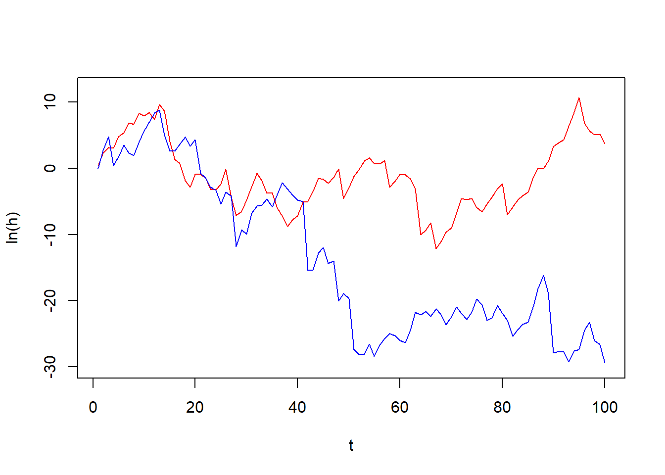
\[ \mathbb{V}ar\left\{\mathscr{V}_t/\lambda \right\} = \frac{1}{\lambda^2} \mathbb{V}ar\left\{\mathscr{V}_t \right\} = \frac{1}{\lambda^2}\frac{2\nu}{(1+\nu)^2(3+\nu)} = 16e^{2\gamma}e^{2\psi\left(\frac{\nu+1}{2}\right)}\frac{2\nu}{(1+\nu)^2(3+\nu)} = \frac{32\nu e^{2\gamma + 2\psi\left( \frac{\nu+1}{2} \right)}}{(1+\nu)^2(3+\nu)} \approx \frac{32\nu e^{2\gamma + 2\ln(1+\nu) -2\ln(2) -2/(1+\nu)}}{(1+\nu)^2(3+\nu)} = 8e^{2\gamma}\frac{\nu e^{-2/(1+\nu)}}{3+\nu} \] So \(\lim_{\nu\rightarrow +\infty} \mathbb{V}ar\left\{ \mathscr{V}_t/\lambda \right\} = 8e^{2\gamma}\). This means that the model can not nest the homoskedastic Gaussian AR(1). If this were true, the expected value should be 1 and the variance 0, so that \(h_{t+1} = h_t\). In the following graph I plot a path of \(\ln h_t\) with \(\nu = 3\) and \(80000\).

The model does not nest the homoskedastic case. So, what is the limiting distribution of \(\mathscr{V}_t/\lambda\)?

References

Uhlig, H. (1997). Bayesian vector autoregressions with stochastic volatility. Econometrica: Journal of the Econometric Society, 59-73.
Nelson, D. B. (1990). Stationarity and persistence in the GARCH (1, 1) model. Econometric theory, 6(3), 318-334.