Tests for correct specification of conditional predictive densities

June 20, 2020

I have implemented the statistical tests of Rossi and Sekhposyan (2019) in R. You can find the codes in the following Github repo. Two tests, a Kolmogorov-Smirnov test and an Cràmer-von Mises test, are implemented to assess the correct specification of rolling window conditional distribution out-of-sample forecasts, one and multiple steps ahead.

Thew hole idea of the test is the following: let \(X\) be a random variable with cdf \(F_X\) (with well defined \(F_X^{-1}\)). If we define a new variable \(Y = F_X(X)\), then \(F_Y(y) = \mathbf{P}(Y \leq y) = \mathbf{P}(F_X(X) \leq y) = \mathbf{P}(X \leq F_X^{-1}(y)) = F_X(F_X^{-1}(y)) = y\). The random variable that has \(y\) as CDF is a uniform random variable. This is known as the probability inverse transform.

When forecasting the distribution of the random variable \(X\) if we picked as our forecast it’s true CDF (good job!), when we evaluate the realizations of the random variable using our CDF we should get a uniform random variable. Thus we can test if it indeed follows a uniform distribution. There are three variants of the test one ca use. In the case of one-setp-ahead forecasts one can use the asymptotic critical values reported in Table 1 of Rossi and Sekhposyan (2019). Alternatively if one wants to test a particular set of quantiles that are not reported in Table 1 one can use their Monte-Carlo method, which I implemented in R to obtain the critical values. In the case of multiple-step-ahead forecasts one must use procedure involving block boostrap to correct for the fact that errors might be autocorrelated.

Aplications to Financial Risk Management

Aside from a general application to forecasting it also has a particular application to financial risk management. Expected shortfall is the risk measure at the forefront of Basel III. The accuracy of expected shortfall depends on the accuracy of the predicted distributions, their left tail in fact. Therefore we might want to backtest that the left tail of the predictive distributions is well specified. Unlike Diebold (1998) the test is joint, not pointwise, and is robust to serial correlation of the probability integral transforms (multi-step-ahead forecasts).

Test

Input

The test is implemented in the function RStest which has several arguments:

pits: A vector containing the probability integral transforms (predicted CDF evaluated at it’s realization), thus it’s elements are numeric and in [0, 1]. Elements are ordered from t = R to T, the out-of-sample set.
alpha: significance level, the probability of rejecting the null hypothesis when it is true.
nSim: number of simulations in the calculation of the critical values. Must be a positive integer.
rmin: lower quantile to be tested. Must be in [0,1] and > than rmax.
rmax: upper quantile to be tested. Must be in [0,1] and < than rmin.
step: must be a string, either “one” or “multiple”. The first option implements the second boostrap procedure described in Theorem 2 of Rossi and Sekhposyan (2019) to compute critical values, while the second option implements the procedure described in Theorem 4 of Rossi and Sekhposyan (2019), which is robust to autocorrelation of the probability integral transforms (recommended for multi-step-ahead forecasts).
l: Bootstrap block length. Default is set to [\(P^{1/3}\)], where [⋅] denotes the floor operator, as in all Pannels, except G, of Table 3 in Rossi and Sekhposyan (2019). Boostrap block length must be a positive integer. Specifying the boostrap block length is unnecessary for one-step-ahead forecasts. Although there is no guidance on how to choose l, results seem to be robust to alternative lengths.

Output

The test outputs a list with several objects:

KS_P: Kolmogorov-Smirnov statistic.
KS_alpha: Kolmogorov-Smirnov critical value.
CvM_P: Cràmer-von Mises statistic.
CvM_alpha: Cràmer-von Mises critical value.

The null hypothesis of the correct specification of the conditional distribution can be rejected if the statistic is larger than the critical value.

Example: AR(1)

\[ DGP: y_{t+1} = 0.8 y_{t} + e_{t+1}; \ e_{t+1} \sim \mathcal{N}(0,2) \] What we are going to do here is estimate a model, regression, from data to \(t_0\) to \(t_N\), generate a forecast of the distribution at \(t_{N+1}\) and evaluate the CDF at the realized value \(y_{t+1}\), obtaining values the probability integral transform. Those will be feed into the test in which the null hypothesis is that the whole conditional distribution is well specified.

#Simulate the model, 500 observations take the last 221. 70 to estimate initial model, 150 forecasts.
set.seed(777)
y <- c(0)

for (i in 2:500){
  e <- rnorm(1, mean = 0, sd = sqrt(2))
  y <- c(y, 0.8*y[i-1] + e)
}

y_1 <- y[279:499]
y <- y[280:500]

#Use a rolling window of 50 estimate the mode, evaluate CDF (t+1, a t forecast) at realized value (t+1)

pits <- c()

for (i in 1:150){
  y_reg <- y[(1+i):(70+i)]
  y_1_reg <- y_1[(1+i):(70+i)]
  reg <- lm(y_reg ~ y_1_reg)
  y_forecast <- y[71+i]
  cond_mean <- c(reg$coefficients[1] + reg$coefficients[2]*y[70+i])
  cond_sd <- sd(reg$residuals)
  pits <- c(pits, pnorm(y_forecast, mean = cond_mean, sd = cond_sd))
}

P <- length(pits)
plot(ecdf(pits), main = "")
abline(a = 0, b = 1, col = "blue")
abline(a = 1.34/sqrt(P) , b = 1, col = "red")
abline(a = -1.34/sqrt(P), b = 1, col = "red")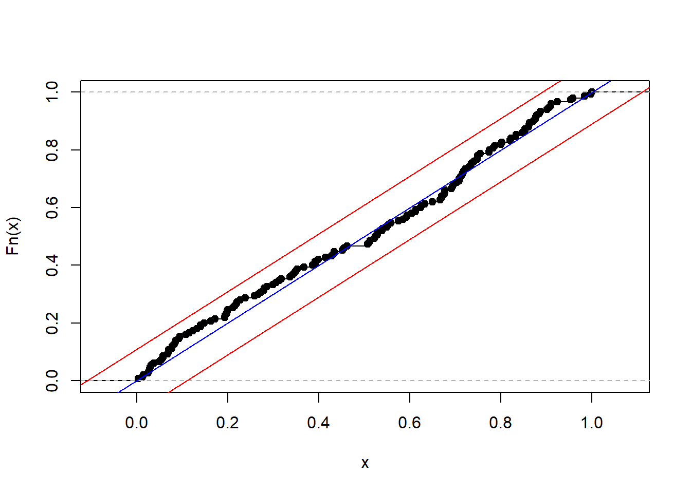

results <- RStest(pits, alpha = 0.05, nSim = 1000, rmin = 0, rmax = 1, step = "one")
print(results)

## $KS_P
## [1] 0.7144345
## 
## $KS_alpha
##      95% 
## 1.379879 
## 
## $CvM_P
## [1] 0.1201941
## 
## $CvM_alpha
##       95% 
## 0.4986979

As an alternative we can also specify a wrong forecast. In this case I picked that we are going to incorrectly assume that the process is white noise and set the mean and the variance to the unconditional mean and variance of the AR(1). We’ll see that the correct specification of the whole distribution is rejected.

pits <- c()

for (i in 1:150){
  y_forecast <- y[71+i]
  cond_mean <- 0/(1-0.8)
  cond_sd <- sqrt(2/(1-0.8^2))
  pits <- c(pits, pnorm(y_forecast, mean = cond_mean, sd = cond_sd))
}

P <- length(pits)
plot(ecdf(pits), main = "")
abline(a = 0, b = 1, col = "blue")
abline(a = 1.34/sqrt(P) , b = 1, col = "red")
abline(a = -1.34/sqrt(P), b = 1, col = "red")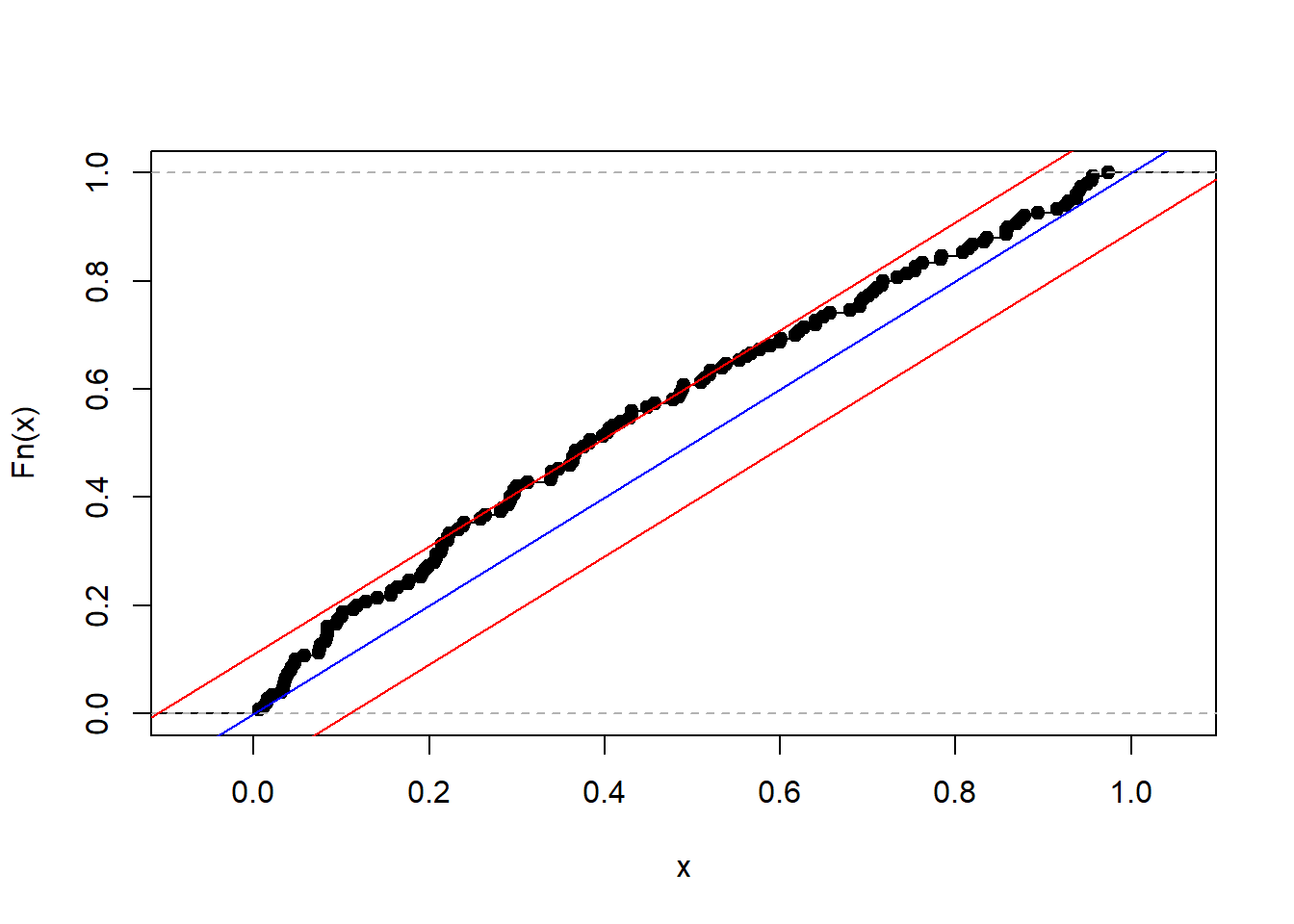

results <- RStest(pits, alpha = 0.05, nSim = 1000, rmin = 0, rmax = 1, step = "one")
print(results)

## $KS_P
## [1] 1.579921
## 
## $KS_alpha
##      95% 
## 1.347423 
## 
## $CvM_P
## [1] 0.9243886
## 
## $CvM_alpha
##       95% 
## 0.4512982

References

Rossi, Barbara, and Tatevik Sekhposyan. “Alternative tests for correct specification of conditional predictive densities.” Journal of Econometrics 208.2 (2019): 638-657.