Growth-at-Risk IMF Tool
June 21, 2020
The International Monetary Fund (IMF) has been using Growth-at-Risk, a macro-econometric tool developed by them to assess risks to economic growth, in several article IV country reports (Albania, Portugal and Singapore 2018), Chapter 2 of the IMF Global Financial Conditions Report since October 2017 and so on. The tool is built taking the methodology developed in the AER April 2019 paper Vulnerable Growth.
I have several doubts about the statistical procedures used and the interpretation of the results in the original AER paper but I want to keep the post short. This tool has been assessed by the paper “Backtesting Global Growth-at-Riskâ€, where they show that the Growth-at-Risk tool procedure consistently fails to beat a simple GARCH model.
Two of the crucial steps described in the AER paper are the following:
- Obtain conditional quantile forecasts of GDP growth using quantile regression:
\[ \hat{Q}_{y_{t+h}|x_t}(\tau|x_t) = x_t \hat{\beta}_\tau \]
- Fit a skew t-distribution to the four fitted values of the quantile regression by minimizing the squared distance between the skewed student t-distribution quantiles and the regression quantiles.
\[ \{\hat{\mu}_{t+h}, \hat{\sigma}_{t+h}, \hat{\alpha}_{t+h}, \hat{\nu}_{t+h} \} = \underset{\mu, \sigma, \alpha, \nu}{argmin} \sum_{\tau}\left( \hat{Q}_{y_{t+h}|x_t}(\tau|x_t) - F^{-1}(\tau; \mu, \sigma, \alpha, \nu) \right)^2 \]
where \(F(·)\) is the CDF of a skewed t-distribution.
Now, if we go the technical appendix of the Growth-at-Risk IMF tool Github repository, in footnote 11 (section about unconstrained optimization) one can find the following:
To avoid that the t-skew parametrization converges towards a Gaussian (infinite degrees of freedom), the tool anchors the degrees of freedom at 2.
Yet, there seems to be no reason why the degrees of freedom should be fixed at 2, and no reason to prevent the distribution to converge towards a Gaussian if the data indicates so. How does this affect the distributions estimated? Is it a big change? This are the questions I’m now going to answer. To do that I will replicate Figure 8. Probability Densities (one-quarter-ahead GDP and NFCI distributions only) of the AER paper first with completely unconstrained optimization, like the AER paper, and then fixing the degrees of freedom to 2.
| location | scale | skewness | freedom | |
| Q2.2006 | 1.921 | 2.707 | 1.802 | 30 |
| Q4.2008 | 2.117 | 2.614 | -0.860 | 3 |
| Q4.2014 | 2.357 | 2.506 | 2.030 | 30 |
| location | scale | skewness | freedom | |
| Q2.2006 | 3.390 | 1.188 | 0.325 | 2 |
| Q4.2008 | 1.467 | 1.975 | -0.521 | 2 |
| Q4.2014 | 3.713 | 1.078 | 0.377 | 2 |
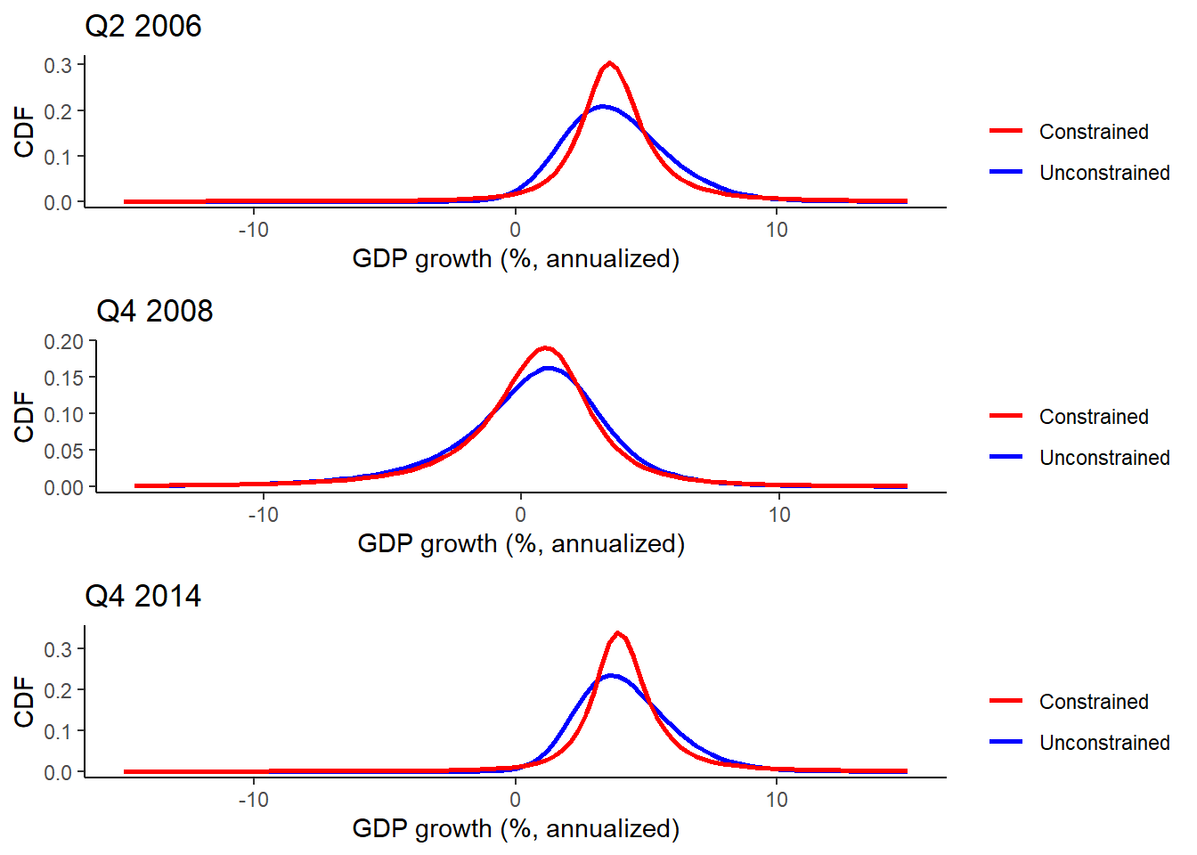
As we can see, all constrained distributions put a higher weight to values around the center of the distribution compared to unconstrained distributions. This is even limited by the fact that in the AER paper degrees of freedom are not allowed to be larger than 30. Now that we have analyzed the changes, why did the authors of the tool make this conscious choice? I believe that as the original MatLab routine incorporated a grid search for the degrees of freedom that took quite some time, and that Python is not a very fast language, the authors opted to drop this computationally costly grid search and set the degrees of freedom to 2. Python is intended to be the back-end for a Growth-at-Risk Excel plugin.
Note: Even if the graphs in blue (unconstrained) don’t seem, visually, to exactly match the AER Figure 8, the printed parameters of the distributions are identical to those found in the replication codes.
References
Adrian, T., Boyarchenko, N., & Giannone, D. (2019). Vulnerable growth. American Economic Review, 109(4), 1263-89.
Brownlees, Christian T. and Souza, Andre B.M., Backtesting Global Growth-at-Risk (September 29, 2019). Available at SSRN: https://ssrn.com/abstract=3461214 or http://dx.doi.org/10.2139/ssrn.3461214