Acerbi & Szekely Unconditional Expected Shortfall Test

Input

##         
##         X_obs (np.array): Numpy array of size 1xT containing the actual 
##                           realization of the portfolio return.
##                           
##         X (function): Function that simulates (outputs) a realization of the 
##                       portfolio return under H0: 
##                       X^s = (X_1^s, X_2^s,..., X_T^s), with X_t^s ~ P_t for all
##                       t = 1 to T.
##                       Output should be a numpy array of 1xT.
##                       
##         VaRLevel (float): Number describing the level of the VaR, say 0.05 for 
##                           95% or 0.01 for 99%.
##         
##         VaR (np.array): Numpy array of size 1xT containing the projected 
##                         Value-at-Risk estimates for t = 1 to T at VarLevel.
##                         VaR must not be reported in its positive values, but
##                         rather in its actual values, usually negative.
##                         
##         ES (np.array): Numpy array of size 1xT containing the projected
##                        Expected Shortfall estimates for t = 1 to T at VaRLevel.
##                        ES must not be reported in its positive values, but 
##                        rather in its actual values, usually negative.
## 
##         nSim (int): Number of Monte Carlo simulations, scenarios, to obtain the
##                     distribution of the statistic under the null hypothesis of 
##                     P_t^[VaRLevel] = F_t^[VaRLevel].
##                     
##         alpha (float): Number in [0, 1] denoting the Type I error, the 
##                        significance level threshold used to compute the 
##                        critical value. Default set at 5%
##                        
##         print_results (boolean): Boolean for whether results should be printed. 
## 

Examples

We run the test under two different scenarios. In the first scenario the portfolio returns are generated from a normal distribution mixture such that there is a bump in the left tail compared to a normal distribution. In the second case the portfolio returns are generated form a normal.

Then returns are always assumed to follow a normal distribution with the sample mean and variance. We can observe that the Value at Risk and Expected Shortfall estimates at 95% are strongly rejected in the first case but not in the second case.

The first case is:

\[ TDGP: r_t \sim \ \ \text{i.i.d} \ \ \mathbb{1}_{\phi_t = 0} \mathcal{N}(\mu_{standard}, \sigma_{stress}) + \mathbb{1}_{\phi_t = 1} \mathcal{N}(\mu_{stress}, \sigma_{stress}) \] where \(\phi_t \sim\) i.i.d \(Bernoulli(p)\).

\[ Model: r_t \sim \ \ \text{i.i.d} \ \ \mathcal{N}(\hat{\mu}, \hat{\sigma}) \]

## ----------------------------------------------------------------
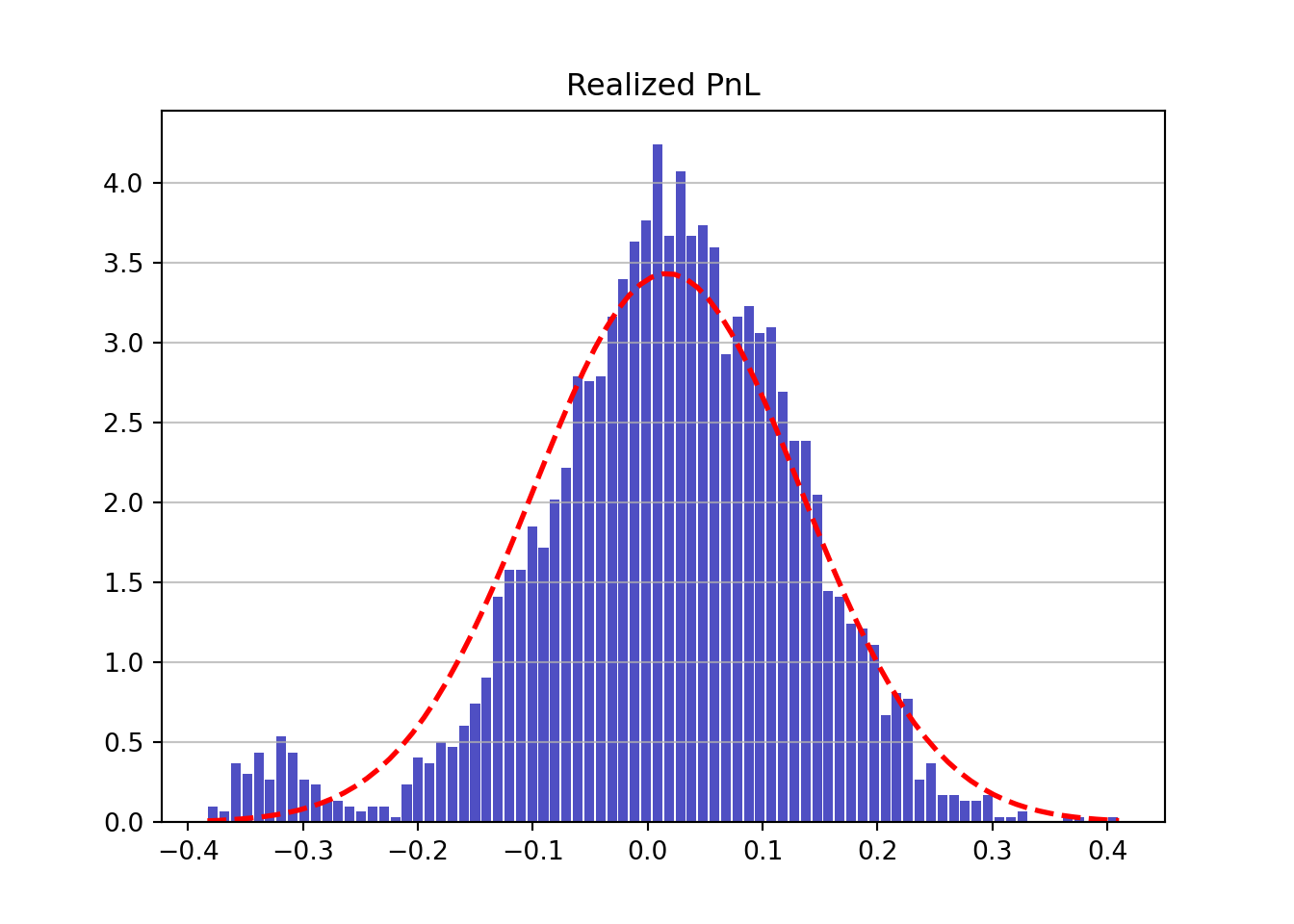
##    Direct/Unconditional Expected Shortfall Test by Simulation   
## ----------------------------------------------------------------
## Number of observations: 3000
## Number of VaR breaches: 156
## Expected number of VaR breaches: 150.0
## ES Statistic: -0.29866795648622135
## Expected ES Statistic: 0
## Critical Value at α = 0.05: -0.13574459537691758
## p-value: 0.0002
## Number of Monte Carlo simulations: 10000
## ----------------------------------------------------------------

The second case is:

\[ TDGP: r_t \sim \ \ \text{i.i.d} \ \ \mathcal{N}(\mu_{standard}, \sigma_{standard}) \]

\[ Model: r_t \sim \ \ \text{i.i.d} \ \ \mathcal{N}(\hat{\mu}, \hat{\sigma}) \]

## ----------------------------------------------------------------
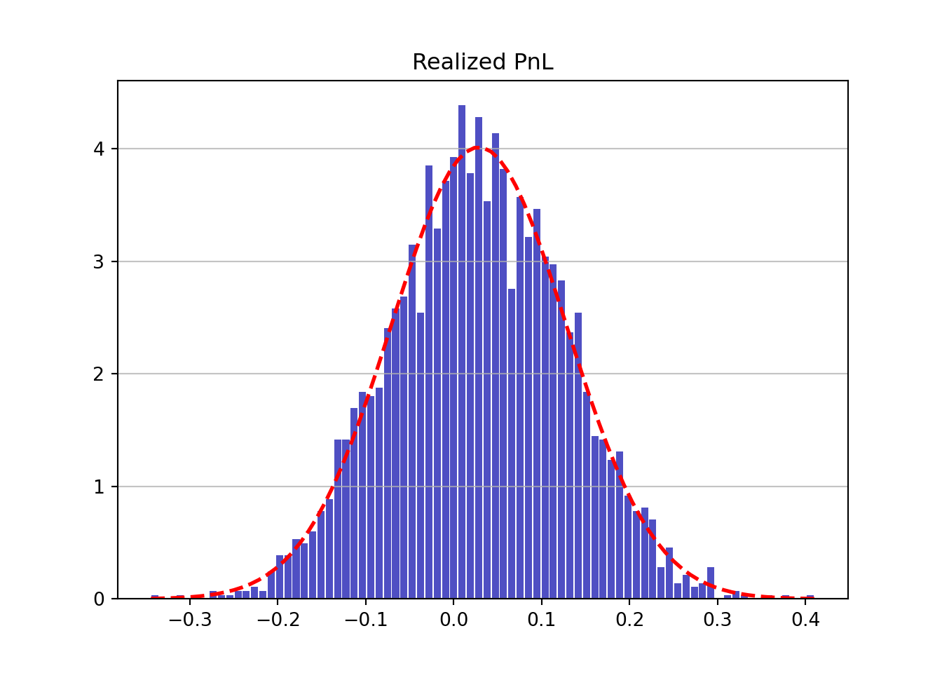
##    Direct/Unconditional Expected Shortfall Test by Simulation   
## ----------------------------------------------------------------
## Number of observations: 3000
## Number of VaR breaches: 144
## Expected number of VaR breaches: 150.0
## ES Statistic: 0.05483829919134353
## Expected ES Statistic: 0
## Critical Value at α = 0.05: -0.13545881827342304
## p-value: 0.7471
## Number of Monte Carlo simulations: 10000
## ----------------------------------------------------------------

References

Acerbi, Carlo, and Balazs Szekely. “Back-testing expected shortfall.” Risk 27.11 (2014): 76-81.